Markov Decision Processes

CSCI 4511/6511

Joe Goldfrank

Announcements

• Homework Four: 29 Mar
• Project Scope: 5 Apr
• Homework 3: Resubmission
  • +80 pts from original
  • Can’t exceed 100
  • Due 10 Apr (hard stop)

Markov Chains

Markov property:

\(P(X_{t} | X_{t-1},X_{t-2},...,X_{0}) = P(X_{t} | X_{t-1})\)

“The future only depends on the past through the present.”

• State \(X_{t-1}\) captures “all” information about past
• No information in \(X_{t-2}\) (or other past states) influences \(X_{t}\)

What Even Is State?

Random Walk:

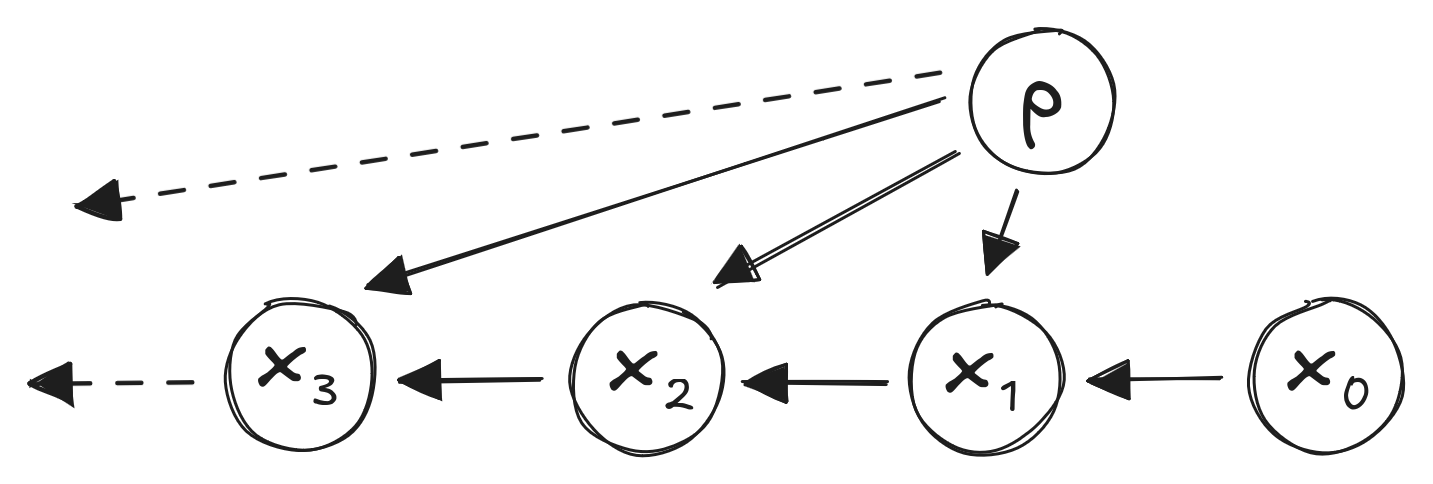
• Start with some amount of money, flip coin:
  • Heads: Gain $1
  • Tails: Lose $1
• \(x_t\): Money
• \(p\): Coin flip probability

What Even Is State?

The Same Random Walk:

• \(x_t\): tuple (Money, coin flip probability)
• Markov Property satisfied

State Transitions

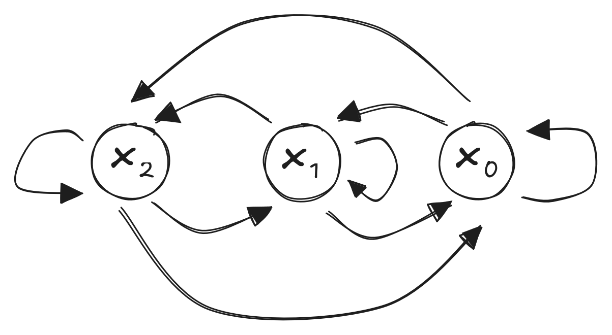
Stochastic matrix \(P\)

\[ P = \begin{bmatrix} P_{1,1} & \dots & P_{1,n}\\ \vdots & \ddots & \\ P_{n, 1} & & P_{n,n} \end{bmatrix} \]

• All rows sum to 1
• Discrete state spaces implied

State Transitions

State Transitions

• State: Full state \(x\) is row vector
  • Each entry represents one state
• Example: three states representing weather
  • Clear, Clouds, Rain
  • \(x_t = \begin{bmatrix}1 & 0 & 0\end{bmatrix} \rightarrow\) Clear
  • \(x_t = \begin{bmatrix}0 & 1 & 0\end{bmatrix} \rightarrow\) Clouds
  • \(x_t = \begin{bmatrix}0 & 0 & 1\end{bmatrix} \rightarrow\) Rain

State Transitions

\(x_{t+1} = x_t P\)

\(x_0 = \begin{bmatrix}1 & 0 & 0\end{bmatrix}\) and \(P = \begin{bmatrix} 0.5 & 0.4 & 0.1 \\ 0.3 & 0.4 & 0.3 \\ 0.1 & 0.7 & 0.2 \end{bmatrix}\)

\(x_{1} = \begin{bmatrix}1 & 0 & 0\end{bmatrix} \begin{bmatrix} 0.5 & 0.4 & 0.1 \\ 0.3 & 0.4 & 0.3 \\ 0.1 & 0.7 & 0.2 \end{bmatrix} = \begin{bmatrix}0.5 & 0.4 & 0.1\end{bmatrix}\)

State Transitions

\(x_{1} = \begin{bmatrix}0.5 & 0.4 & 0.1\end{bmatrix}\)

Probabilities of being in each state: Clear, Clouds, Rain

\(x_{2} = \begin{bmatrix}0.5 & 0.4 & 0.1\end{bmatrix} \begin{bmatrix} 0.5 & 0.4 & 0.1 \\ 0.3 & 0.4 & 0.3 \\ 0.1 & 0.7 & 0.2 \end{bmatrix}\)

\(= \begin{bmatrix}0.38 & 0.43 & 0.35\end{bmatrix}\)

numpy

• Use the matrix multiplication operator: @
• Altneratively: numpy.matmul

import numpy as np
P = np.array([[0.5, 0.4, 0.1], 
              [0.3, 0.4, 0.3], 
              [0.1, 0.7, 0.2]])

x0 = np.array([1, 0, 0])

x1 = x0 @ P
print(x1)

[0.5 0.4 0.1]

Stationary Behavior

• “Long run” behavior of Markov chain

\(x_0 P^k\) for large \(k\)

• “Stationary state” \(\pi\) such that:

\(\pi = \pi P\)

• Row eigenvector for \(P\) for eigenvalue 1
• 😌

Stationary Behavior (numpy)

\(P^k\)

import numpy as np
P = np.array([[0.5, 0.4, 0.1], 
              [0.3, 0.4, 0.3], 
              [0.1, 0.7, 0.2]])

x0 = np.array([1, 0, 0])
print(x0 @ P @ P @ P @ P @ P @ P @ P @ P @ P)
x1 = np.array([0, 1, 0])
print(x1 @ P @ P @ P @ P @ P @ P @ P @ P @ P)

[0.32144092 0.46427961 0.21427948]
[0.32142527 0.46428717 0.21428756]

Eigenvector

a = np.linalg.eig(P.T).eigenvectors[:,0] # row eigenvector
pi = a/sum(a) # normalized
print(pi)

[0.32142857 0.46428571 0.21428571]

Absorbing States

• State that cannot be “escaped” from
  • Example: gambling \(\rightarrow\) running out of money

\(P = \begin{bmatrix} 0.5 & 0.3 & 0.1 & 0.1 \\ 0.3 & 0.4 & 0.3 & 0 \\ 0.1 & 0.6 & 0.2 & 0.1 \\ 0 & 0 & 0 & 1 \end{bmatrix}\)

• Non-absorbing states: “transient” states

Communication

• Sub-classes

\(P = \begin{bmatrix} 0.5 & 0.3 & 0.2 & 0 & 0 \\ 0.3 & 0.4 & 0.3 & 0 & 0\\ 0.1 & 0.6 & 0.2 & 0.1 & 0 \\ 0 & 0 & 0 & 0.6 & 0.4 \\ 0 & 0 & 0 & 0.3 & 0.7 \end{bmatrix}\)

• Examples?

Non-Discrete Cases

Gaussian random walk:

\(x_{t+1} = x_t + \mathcal{N}(0,1)\)

• Markov property?
• “Long-run” behavior?

\(\mathcal{N}(\mu_a,\sigma_a^2) + \mathcal{N}(\mu_b,\sigma_b^2) = \mathcal{N}(\mu_a + \mu_b,\sigma_a^2 + \sigma_b^2)\)

😌

Outcomes¹

• Each state associated with some “reward”
  • Spend one time step in state \(\rightarrow\) reward collected
• Future rewards discounted

Discounting:

• \(\$1.00\) today bears interest \(\rightarrow\) \(\$1.05\) next year
• \(\$1.00\) next year is worth \(\frac{1}{1.05} \approx \$0.95\) today
• Rationale: resources today are productive
  • Build things for the future

1. Everyone has them

Markov Reward Process

• Reward function \(R_s = E[R_{t+1} | S_t = s]\):
  • Reward for being in state \(s\)
• Discount factor \(\gamma \in [0, 1]\)

\(U_t = \sum_k \gamma^k R_{t+k+1}\)

Example

States: Sales Volume

\(P = \begin{matrix} Low \\ Medium \\ High \end{matrix} \begin{bmatrix} 0.4 & 0.5 & 0.1 \\ 0.2 & 0.6 & 0.2 \\ 0.8 & 0.2 & 0 \end{bmatrix}\)

Rewards:

\(R = \begin{bmatrix} 1 \\ 2.5 \\ 5 \end{bmatrix} \quad \quad \gamma = 0.85\)

Example

Reward for being in state \(x_0 = \begin{bmatrix}0 & 1 & 0\end{bmatrix}\):

\(R_1 = x_0 R = \begin{bmatrix}0 & 1 & 0\end{bmatrix}\begin{bmatrix} 1 \\ 2.5 \\ 5 \end{bmatrix} = 2.5\)

State transition:

\(x_1 = \begin{bmatrix}0 & 1 & 0\end{bmatrix} \begin{bmatrix} 0.4 & 0.5 & 0.1 \\ 0.2 & 0.6 & 0.2 \\ 0.8 & 0.2 & 0 \end{bmatrix} = \begin{bmatrix}0.2 & 0.6 & 0.2\end{bmatrix}\)

\(R_2 = x_1 R = \begin{bmatrix}0.2 & 0.6 & 0.2\end{bmatrix}\begin{bmatrix} 1 \\ 2.5 \\ 5 \end{bmatrix} = 2.7\)

Discounted reward: \(2.7 \cdot \gamma^1 = 2.7\cdot0.85 = 2.295\)

Value Function

\(U_t = \sum_k \gamma^k R_{t+k+1}\)

\(U(s_t) = E\left[R_{t+1} + \gamma U(s_{t+1})\right]\)

\(U(s) = R_{s} + \gamma \sum\limits_{s' \in S} P_{s,s'} U(s')\)

\(U = R + \gamma P U\)

\((I-\gamma P) U = R\)

\(U = (I-\gamma P)^{-1} R\)

Decisions¹

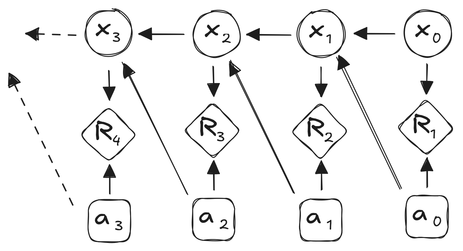
• Markov Decision Process:
  • Actions \(a_t\)

1. Some people make them.

The Markov Decision Process

• Transition probabilities depend on actions

Markov Process:

\(s_{t+1} = s_t P\)

Markov Decision Process (MDP):

\(s_{t+1} = s_t P^a\)

Rewards: \(R^a\) with discount factor \(\gamma\)

Mathematical Notation 😔

• \(P^a\) indicates transition matrix \(P\) associated with action \(a\)
  • Does not mean \(P\) raised to some power
  • We’ve used \(P^k\) for \(P\) raised to the power of \(k\)
• \(P_{i,j}\) indicates transition probability from state \(s_i\) to state \(s_j\)
• \(P_{s,s'}\) indicates transition probability from state \(s\) to state \(s'\)

Alternatively:

• \(T(s' | s, a)\) – transition matrix from \(s\) to \(s'\) given action \(a\)

MDP Example

• States: Sales Volume
• Actions: \(a_0, a_1\)

\(P^0 = \begin{matrix} Low \\ Medium \\ High \end{matrix} \begin{bmatrix} 0.4 & 0.5 & 0.1 \\ 0.2 & 0.6 & 0.2 \\ 0.8 & 0.2 & 0 \end{bmatrix} \quad P^1 = \begin{matrix} Low \\ Medium \\ High \end{matrix} \begin{bmatrix} 0.2 & 0.6 & 0.2 \\ 0.1 & 0.6 & 0.3 \\ 0.5 & 0.4 & 0.1 \end{bmatrix}\)

• Rewards: product of state and action

\(R^0 = \begin{bmatrix} 1 \\ 2.5 \\ 5 \end{bmatrix} R^1 = \begin{bmatrix} 0 \\ 1.5 \\ 4 \end{bmatrix} \quad \quad \gamma = 0.85\)

• What does this example model?

MDP - Policies

• Agent function
  • Actions conditioned on states

\(\pi(s) = P[A_t = a | s_t = s]\)

• Can be stochastic
  • Usually deterministic
  • Usually stationary

MDP - Policies

State value function \(U^\pi\):¹

\(U^\pi(s) = E_\pi[U_t | S_t = s]\)

State-action value function \(Q^\pi\):²

\(Q^\pi(s,a) = E_\pi[U_t | S_t = s, A_t = a]\)

Notation: \(E_\pi\) indicates expected value under policy \(\pi\)

1. Often simply called “value function”

2. Often simply called “action value function”

Bellman Expectation

Value function:

\(U^\pi(s) = E_\pi[R_{t+1} + \gamma U^\pi (S_{t+1}) | S_t = s]\)

Action-value fuction:

\(Q^\pi(s, a) = E_\pi[R_{t+1} + \gamma Q^\pi(S_{t+1}, A_{t+1}) | S_t = s, A_t =a]\)

Bellman Expectation

Value function:

\(U^\pi(s) = E_\pi[R_{t+1} + \gamma U^\pi (S_{t+1}) | S_t = s]\)

Action-value fuction:

\(Q^\pi(s, a) = E_\pi[R_{t+1} + \gamma Q^\pi(S_{t+1}, A_{t+1}) | S_t = s, A_t =a]\)

Policy Evaluation

• How good is some policy \(\pi\)?

\(U^\pi_1(s) = R(s, \pi(s))\)

\(U^\pi_{k+1}(s) = R(s, \pi(s)) + \gamma \sum \limits_{s^{'}} T(s' | s, \pi(s)) U_k^\pi(s')\)

• Exact solution (matrix form):

\(U^\pi = R^\pi + \gamma T^\pi U^\pi\)

\(U^\pi = (I-\gamma T^\pi)^{-1}R^\pi\)

Optimal Policies 😌

• There will always be an optimal policy
  • For all MDPs!
• Policy ordering:
  • \(\pi \geq \pi' \;\) if \(\; U^\pi(s) \geq U^{\pi'}(s), \; \forall s\)
• Optimal policy:
  • \(\pi* \geq \pi, \; \forall \pi\)
  • \(U^{\pi*}(s) = U^*(s)\) and \(Q^{\pi*}(s) = Q^*(s)\)

Optimal Policies

• Optimal policy \(\pi^*\) maximizes expected utility from state \(s\):
  • \(\pi^*(s) = \mathop{\operatorname{arg\,max}}\limits_a U^*(s)\)
• Value function:
  • \(U^*(s) = \max_a U^*(s)\)

Optimal Policies

• Action-value function:
  • \(Q(s, a) = R(s, a) + \gamma \sum \limits_{s'} T(s' | s, a) U(s')\)
• Greedy policy given some \(U(s)\):
  • \(\pi(s) = \mathop{\operatorname{arg\,max}}\limits_a Q(s,a)\)

Partial Bellman Equation

Decision: \[U^*(s) = \max_a Q^*(s,a)\]

Partial Bellman Equation

Stochastic: \[Q^*(s, a) = R(s, a) + \gamma \sum \limits_{s'} T(s' | s, a) U^*(s')\]

Bellman Equation

\[U^*(s) = \max_a R(s, a) + \gamma \sum \limits_{s'} T(s' | s, a) U^*(s')\]

Bellman Equation

\[Q^*(s, a) = R(s, a) + \gamma \sum \limits_{s'} T(s' | s, a) \max_a Q^*(s', a')\]

How To Solve It

• No closed-form solution
  • Optimal case differs from policy evaluation

Iterative Solutions:

• Value Iteration
• Policy Iteration

Reinforcement Learning

Dynamic Programming

• Assumes full knowledge of MDP
• Decompose problem into subproblems
  • Subproblems recur
• Bellman Equation: recursive decomposition
• Value function caches solutions

Iterative Policy Evaluation

Iteratively, for each algorithm step \(k\):

\(U_{k+1}(s) = \sum \limits_{a \in A}\left(R(s, a) + \gamma \sum \limits_{s'\in S} T(s' | s, a) U_k(s') \right)\)

• “Bellman Backup”

Policy Iteration

Algorithm:

• Until convergence:
  • Evaluate policy
  • Select new policy according to greedy strategy

Greedy strategy:

\[\pi'(s) = \mathop{\operatorname{arg\,max}}\limits_a Q(s,a)\]

Unpacking the Notation

\[\pi(s) = \mathop{\operatorname{arg\,max}}\limits_a Q(s,a)\]

• \(\pi'(s)\)
  • New policy \(\pi'\)
  • New policy is a function of state: \(\pi'(s)\)
• \(Q(s,a)\)
  • Value of state, action pair\((s, a)\)
• Policy as function of state \(s\)
  • Looks over all actions at each state
  • Chooses action with highest value (argmax)

Policy Iteration

Previous step:

• \(Q^\pi(s,\pi(s))\)

Current step:

• \(Q^\pi(s, \pi' (s)) \gets \max \limits_a Q^\pi(s,a) \geq Q^\pi(s, \pi(s))\)
  • \(= U^\pi(s)\)

Policy Iteration

Convergence:

• \(Q^\pi(s, \pi' (s)) = \max \limits_a Q^\pi(s,a) = Q^\pi(s, \pi(s))\)
  • \(= U^\pi(s)\)

Convergence

• Does our policy need to converge to \(U^\pi\) ?
  • \(U^\pi\) represents value
  • We care about policy¹

Modified Policy Iteration:

• \(\epsilon\)-convergence
• \(k\)-iteration policy evaluation
• \(k = 1\): Value Iteration

1. We do also care about value.

Value Iteration

Optimality:

• Given state \(s\), states \(s'\) reachable
• Optimal policy \(\pi(s)\) achieves optimal value:
  • \(U^\pi(s') = U^*(s')\)

Assume:

• We have \(U^*(s')\)
• We want \(U^*(s)\)

Value Iteration

One-step lookahead:

\[U^*(s) \gets \max \limits_a \left( R(s,a) + \gamma \sum \limits_s' T(s'|s, a) U^*(s') \right)\]

• Apply updates iteratively
• Use current \(U(s')\) as “approximation” for \(U^*(s')\)
• That’s the algorithm.
• Extract policy from values after completion.

Value Iteration Illustrated

\[U_{k+1}(s) \gets \max \limits_a \left( R(s,a) + \gamma \sum \limits_s' T(s'|s, a) U_k(s') \right)\]

Synchronous Value Iteration…

\[U_{k+1}(s) \gets \max \limits_a \left( R(s,a) + \gamma \sum \limits_s' T(s'|s, a) U_k(s') \right)\]

• \(U_k(s)\) held in memory until \(U_{k+1}(s)\) computed
• Effectively requires two copies of \(U\)

Asynchronous Value Iteration

• Updating \(U(s)\) for one state at a time:

\[U(s) \gets \max \limits_a \left( R(s,a) + \gamma \sum \limits_s' T(s'|s, a) U(s) \right)\]

• Ordering of states can vary
• Converges if all states are updated
  • …and if algorithm runs infinitely

References

• Richard S. Sutton and Andrew G. Barto. Reinforcement Learning: An Introduction. 2nd Edition, 2018.

• Mykal Kochenderfer, Tim Wheeler, and Kyle Wray. Algorithms for Decision Making. 1st Edition, 2022.

• John G. Kemeny and J. Laurie Snell, Finite Markov Chains. 1st Edition, 1960.

• Stanford CS234 (Emma Brunskill)

• UCL Reinforcement Learning (David Silver)

• Stanford CS228 (Mykal Kochenderfer)