MDPs and Reinforcement Learning

CSCI 4511/6511

Joe Goldfrank

Announcements

• Homework Three:
  • Turn in for 75% credit max through 25 Apr (hard deadline)
• Homework Four: Today
• Project Scope: 6 Apr

Markov Chains

Markov property:

\(P(X_{t} | X_{t-1},X_{t-2},...,X_{0}) = P(X_{t} | X_{t-1})\)

“The future only depends on the past through the present.”

• State \(X_{t-1}\) captures “all” information about past
• No information in \(X_{t-2}\) (or other past states) influences \(X_{t}\)

Markov Reward Process

• Reward function \(R_s = E[R_{t+1} | S_t = s]\):
  • Reward for being in state \(s\)
• Discount factor \(\gamma \in [0, 1]\)

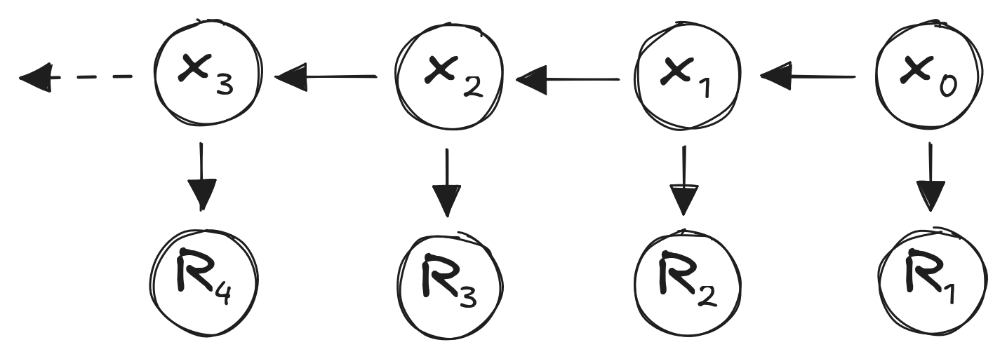
\(U_t = \sum_k \gamma^k R_{t+k+1}\)

Decisions¹

• Markov Decision Process:
  • Actions \(a_t\)

1. Some people make them.

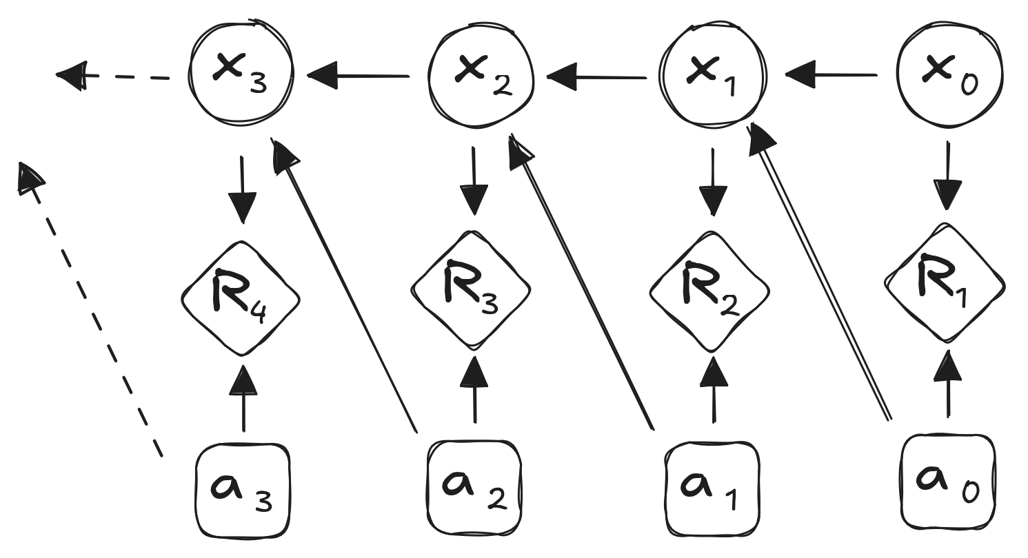
The Markov Decision Process

• Transition probabilities depend on actions

Markov Process:

\(s_{t+1} = s_t P\)

Markov Decision Process (MDP):

\(s_{t+1} = s_t P^a\)

Rewards: \(R^a\) with discount factor \(\gamma\)

MDP - Policies

• Agent function
  • Actions conditioned on states

\(\pi(s) = P[A_t = a | s_t = s]\)

• Can be stochastic
  • Usually deterministic
  • Usually stationary

MDP - Policies

State value function \(U^\pi\):¹

\(U^\pi(s) = E_\pi[U_t | S_t = s]\)

State-action value function \(Q^\pi\):²

\(Q^\pi(s,a) = E_\pi[U_t | S_t = s, A_t = a]\)

Notation: \(E_\pi\) indicates expected value under policy \(\pi\)

1. Often simply called “value function”

2. Often simply called “action value function”

Bellman Expectation

Value function:

\(U^\pi(s) = E_\pi[R_{t+1} + \gamma U^\pi (S_{t+1}) | S_t = s]\)

Action-value fuction:

\(Q^\pi(s, a) = E_\pi[R_{t+1} + \gamma Q^\pi(S_{t+1}, A_{t+1}) | S_t = s, A_t =a]\)

Bellman Expectation

Value function:

\(U^\pi(s) = E_\pi[R_{t+1} + \gamma U^\pi (S_{t+1}) | S_t = s]\)

Action-value fuction:

\(Q^\pi(s, a) = E_\pi[R_{t+1} + \gamma Q^\pi(S_{t+1}, A_{t+1}) | S_t = s, A_t =a]\)

Understanding these equations lynchpins all of MDPs

Value Function

\(U^\pi(s) = E_\pi[R_{t+1} + \gamma U^\pi (S_{t+1}) | S_t = s]\)

State-Action Value Function

\(Q^\pi(s, a) = E_\pi[R_{t+1} + \gamma Q^\pi(S_{t+1}, A_{t+1}) | S_t = s, A_t =a]\)

Policy Evaluation

• How good is some policy \(\pi\)?

\(U^\pi_1(s) = R(s, \pi(s))\)

\(U^\pi_{k+1}(s) = R(s, \pi(s)) + \gamma \sum \limits_{s^{'}} T(s' | s, \pi(s)) U_k^\pi(s')\)

Optimal Policies 😌

• There will always be an optimal policy
  • For all MDPs!
• Policy ordering:
  • \(\pi \geq \pi' \;\) if \(\; U^\pi(s) \geq U^{\pi'}(s), \; \forall s\)
• Optimal policy:
  • \(\pi* \geq \pi, \; \forall \pi\)
  • \(U^{\pi*}(s) = U^*(s)\) and \(Q^{\pi*}(s) = Q^*(s)\)

Optimal Policies

• Optimal policy \(\pi^*\) maximizes expected utility from state \(s\):
  • \(\pi^*(s) = \mathop{\operatorname{arg\,max}}\limits_a U^*(s)\)
• State value function:
  • \(U^*(s) = \max_a U^*(s)\)

Optimal Policies

• State-action value function:
  • \(Q(s, a) = R(s, a) + \gamma \sum \limits_{s'} T(s' | s, a) U(s')\)
• Greedy policy given some \(U(s)\):
  • \(\pi(s) = \mathop{\operatorname{arg\,max}}\limits_a Q(s,a)\)

Partial Bellman Equation

Decision: \[U^*(s) = \max_a Q^*(s,a)\]

Partial Bellman Equation

Stochastic: \[Q^*(s, a) = R(s, a) + \gamma \sum \limits_{s'} T(s' | s, a) U^*(s')\]

Bellman Equation

\[U^*(s) = \max_a R(s, a) + \gamma \sum \limits_{s'} T(s' | s, a) U^*(s')\]

Bellman Equation

\[Q^*(s, a) = R(s, a) + \gamma \sum \limits_{s'} \max_a \left[T(s' | s, a) Q^*(s', a')\right]\]

How To Solve It

• No closed-form solution
  • Optimal case differs from policy evaluation

Iterative Solutions:

• Value Iteration
• Policy Iteration

Reinforcement Learning

Dynamic Programming

• Assumes full knowledge of MDP
• Decompose problem into subproblems
  • Subproblems recur
• Bellman Equation: recursive decomposition
• Value function caches solutions

Iterative Policy Evaluation

Iteratively, for each algorithm step \(k\):

\(U_{k+1}(s) = \sum \limits_{a \in A}\left(R(s, a) + \gamma \sum \limits_{s'\in S} T(s' | s, a) U_k(s') \right)\)

• Deterministic policy: only one action per state

Policy Iteration

Algorithm:

• Until convergence:
  • Evaluate policy
  • Select new policy according to greedy strategy

Greedy strategy:

\[\pi'(s) = \mathop{\operatorname{arg\,max}}\limits_a Q(s,a)\]

Unpacking the Notation

\[\pi(s) = \mathop{\operatorname{arg\,max}}\limits_a Q(s,a)\]

• \(\pi'(s)\)
  • New policy \(\pi'\)
  • New policy is a function of state: \(\pi'(s)\)
• \(Q(s,a)\)
  • Value of state, action pair\((s, a)\)
• Policy as function of state \(s\)
  • Looks over all actions at each state
  • Chooses action with highest value (argmax)

Policy Iteration

Previous step:

• \(Q^\pi(s,\pi(s))\)

Current step:

• \(Q^\pi(s, \pi' (s)) \gets \max \limits_a Q^\pi(s,a) \geq Q^\pi(s, \pi(s))\)
  • \(= U^\pi(s)\)

Policy Iteration

Convergence:

• \(Q^\pi(s, \pi' (s)) = \max \limits_a Q^\pi(s,a) = Q^\pi(s, \pi(s))\)
  • \(= U^\pi(s)\)

Convergence

• Does our policy need to converge to \(U^\pi\) ?
  • \(U^\pi\) represents value
  • We care about policy¹

Modified Policy Iteration:

• \(\epsilon\)-convergence
• \(k\)-iteration policy evaluation
• \(k = 1\): Value Iteration

1. We do also care about value.

Value Iteration

Optimality:

• Given state \(s\), states \(s'\) reachable
• Optimal policy \(\pi(s)\) achieves optimal value:
  • \(U^\pi(s') = U^*(s')\)

Assume:

• We have \(U^*(s')\)
• We want \(U^*(s)\)

Value Iteration

One-step lookahead:

\[U^*(s) \gets \max \limits_a \left( R(s,a) + \gamma \sum \limits_s' T(s'|s, a) U^*(s') \right)\]

• Apply updates iteratively
• Use current \(U(s')\) as “approximation” for \(U^*(s')\)
• That’s it. That’s the algorithm.
• Extract policy from values after completion.

Synchronous Value Iteration…

\[U_{k+1}(s) \gets \max \limits_a \left( R(s,a) + \gamma \sum \limits_s' T(s'|s, a) U_k(s') \right)\]

• \(U_k(s)\) held in memory until \(U_{k+1}(s)\) computed
• Effectively requires two copies of \(U\)

Asynchronous Value Iteration

• Updating \(U(s)\) for one state at a time:

\[U(s) \gets \max \limits_a \left( R(s,a) + \gamma \sum \limits_s' T(s'|s, a) U(s) \right)\]

• Ordering of states can vary
• Converges if all states are updated
  • …and if algorithm runs infinitely

Monte Carlo Tree Search

Multi-Armed Bandits

• Slot machine with more than one arm
• Each pull has a cost
• Each pull has a payout
• Probability of payouts unknown
• Goal: maximize reward
  • Time horizon?

Solving Multi-Armed Bandits

😔

Confidence Bounds

• Expected value of reward per arm
  • Confidence interval of reward per arm
• Select arm based on upper confidence bound

• How do we estimate rewards?
  • Explore vs. exploit

Bandit as MDP?

Bandit Strategies

• Upper Confidence Bound for arm \(M_i\):
  • \(UCB(M_i) = \mu_i + \frac{g(N)}{\sqrt{N_i}}\)
  • \(g(N)\) is the “regret”
• Thompson Sampling
  • Sample arm based on probability of being optimal

Monte Carlo Methods

Tree Search

• Forget DFS, BFS, Dijkstra, A*
  • State space too large
  • Stochastic expansion
• Impossible to search entire tree
• Can simulate problem forward in time from starting state

Monte Carlo Tree Search

• Randomly simulate trajectories through tree
  • Complete trajectory
  • No heuristic needed¹
  • Need a model
• Better than exhaustive search?

1. Heuristics can be used.

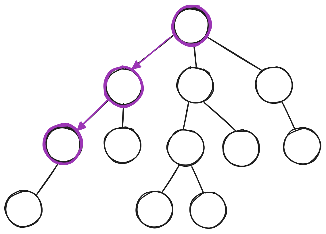
Selection Policy

• Focus search on “important” parts of tree
  • Similar to alpha-beta pruning
• Explore vs. exploit
  • Simulation
  • Not actually exploiting the problem
  • Exploiting the search

Monte Carlo Tree Search

• Choose a node
  • Explore/exploit
  • Choose a successor
  • Continue to leaf of search tree
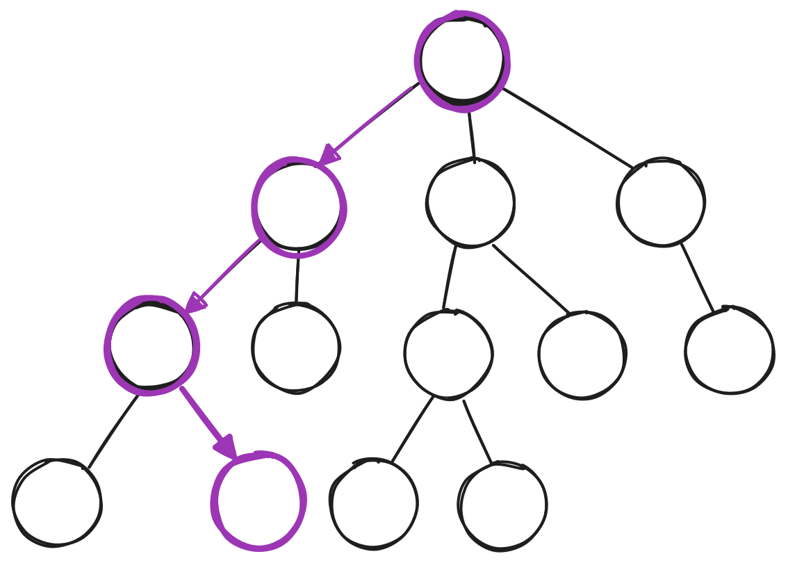
• Expand leaf node
• Simulate result until completion
• Back-propagate results to tree

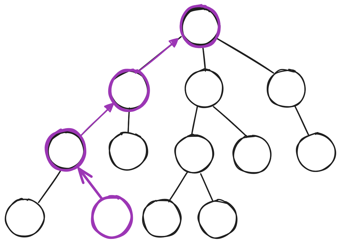
Monte Carlo Tree Search

Selection/Search

Monte Carlo Tree Search

Expansion

Monte Carlo Tree Search

Simulation/Rollout

Monte Carlo Tree Search

Back-Propagation

Upper Confidence Bounds for Trees (UCT)

• MDP: Maximize \(Q(s, a) + c\sqrt{\frac{\log{N(s)}}{N(s,a)}}\)
  • \(Q\) for state \(s\) and action \(a\)
• POMDP: Maximize \(Q(h, a) + c\sqrt{\frac{\log{N(h)}}{N(h,a)}}\)
  • \(Q\) for history \(h\) and action \(a\)
  • History: action/observation sequence
• \(c\) is exploration bonus

UCT Search - Algorithm

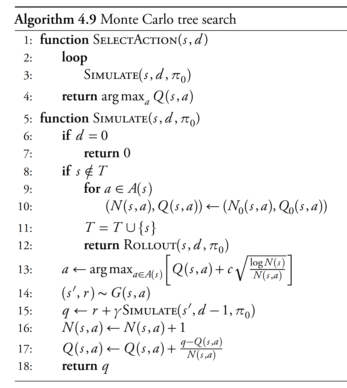
Mykal Kochenderfer. Decision Making Under Uncertainty, MIT Press 2015

Monte Carlo Tree Search - Search

• If current state \(\in T\) (tree states):

  • Maximize: \(Q(s,a) + c\sqrt{\frac{\log N(s)}{N(s,a)}}\)
  • Update \(Q(s,a)\) during search

Monte Carlo Tree Search - Expansion

• State \(\notin T\)
  • Initialize \(N(s,a)\) and \(Q(s,a)\)
  • Add state to \(T\)

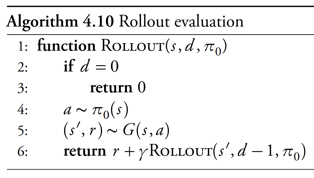
Monte Carlo Tree Search - Rollout

• Policy \(\pi_0\) is “rollout” policy
  • Usually stochastic
  • States not tracked

Model Uncertainty

Erstwhile

• States
• Actions
• Transition model between states, based on actions
• Known rewards

Model Uncertainty

• No model of transition dynamics
• No initial knowledge of rewards

😣

We can learn these things!

Model Uncertainty

Action-value function:

\(Q(s, a) = R(s, a) + \gamma \sum \limits_{s'} T(s' | s, a) U(s')\)

we don’t know \(T\):

\(U^\pi(s) = E_\pi \left[ r_t + \gamma r_{t+1} + \gamma^2 r_{t+2} + \gamma^3 r_{t+3} + ...|s \right]\)

\(Q(s, a) = E_\pi \left[ r_t + \gamma r_{t+1} + \gamma^2 r_{t+2} + \gamma^3 r_{t+3} + ...|s,a \right]\)

Temporal Difference (TD) Learning

• Take action from state, observe new state, reward

\(U(s) \gets U(s) + \alpha \left[ r + \gamma U(s') - U(s)\right]\)

• Update immediately given \((s, a, r, s')\)

• TD Error: \(\left[ r + \gamma U(s') - U(s)\right]\)

  • Measurement: \(r + \gamma U(s')\)
  • Old Estimate: \(U(s)\)

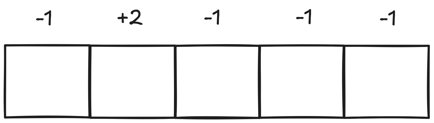
TD Learning - Example

Q-Learning

• \(U^\pi\) gives us utility
• Solving for \(U^\pi\) allows us to pick a new policy

State-action value function: \(Q(s,a)\)

• \(\max_a Q(s,a)\) provides optimal policy
• Goal: Learn \(Q(s,a)\)

Q-Learning

Iteratively update \(Q\):

\(Q(s,a) \gets Q(s,a) +\alpha \left[R + \gamma \max \limits_{a'} Q(s', a') - Q(s,a)\right]\)

• Current state \(s\) and action \(a\)
• Next state \(s'\), next action(s) \(a'\)
• Reward \(R\)
• Discount rate \(\gamma\)
• Learning rate \(\alpha\)

Q-Learning Algorithm

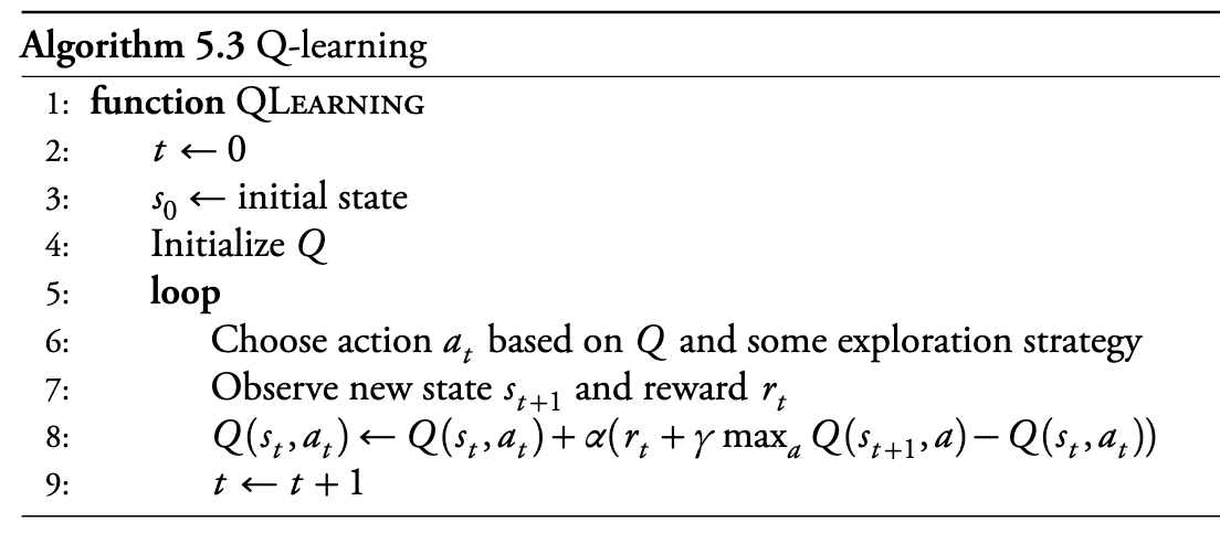
Mykal Kochenderfer. Decision Making Under Uncertainty, MIT Press 2015

Q-Learning Example

Sarsa

Q-Learning: \(Q(s,a) \gets Q(s,a) +\alpha \left[R + \gamma \max \limits_{a'} Q(s', a') - Q(s,a)\right]\)

Sarsa:
\(Q(s,a) \gets Q(s,a) +\alpha \left[R + \gamma Q(s', a') - Q(s,a)\right]\)

Differences?

Sarsa Example

Q-Learning vs. Sarsa

• Sarsa is “on-policy”
  • Evaluates state-action pairs taken
  • Updates policy every step
• Q-learning is “off-policy”
  • Evaluates “optimal” actions for future states
  • Updates policy every step

Exploration vs. Exploitation

• Consider only the goal of learning the optimal policy
  • Always picking “optimal” policy does not search
  • Picking randomly does not check “best” actions
• \(\epsilon\)-greedy:
  • With probability \(\epsilon\), choose random action
  • With probability \(1-\epsilon\), choose ‘best’ action
  • \(\epsilon\) need not be fixed

Eligibility Traces

• Q-learning and Sarsa both propagate Q-values slowly
  • Only updates individual state
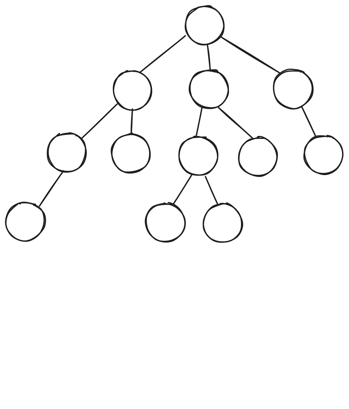
• Recall MCTS:
  • (Also recall that MCTS needs a generative model)

Recall MCTS

Eligibility Traces

• Keep track of what state-action pairs agent has seen
• Include future rewards in past Q-values
• Very useful for sparse rewards
  • Can be more efficient for non-sparse rewards

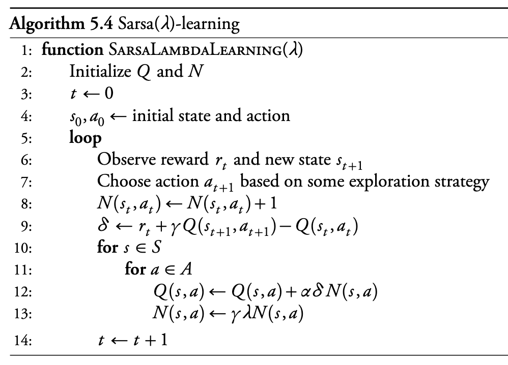
Eligibility Traces

• Keep \(N(s,a)\): “number of times visited”
• Take action \(a_t\) from state \(s_t\):
  • \(N(s_t,a_t) \gets N(s_t,a_t) + 1\)
• Every time step:¹
  • \(\delta = R + \gamma Q(s',a') - Q(s,a)\)
  • \(Q(s,a) \gets \alpha \delta N(s,a)\)
  • \(N(s,a) \gets \gamma \lambda N(s,a)\)
    • Discount factor \(\gamma\)
    • Time decay \(\lambda\)

1. Sarsa algorithm

Sarsa-\(\lambda\)

Sarsa:

• \(Q(s,a) \gets Q(s,a) +\alpha \left[R + \gamma Q(s', a') - Q(s,a)\right]\)

Sarsa-\(\lambda\):

• \(\delta = R + \gamma Q(s',a') - Q(s,a)\)
• \(Q(s,a) \gets \alpha \delta N(s,a)\)

Sarsa-\(\lambda\)

Sarsa-\(\lambda\) Example

Q-\(\lambda\) ?

Q-Learning:
\(\quad \quad Q(s,a) \gets Q(s,a) +\alpha \left[R + \gamma \max \limits_{a'} Q(s', a') - Q(s,a)\right]\)

Sarsa:
\(\quad \quad Q(s,a) \gets Q(s,a) +\alpha \left[R + \gamma Q(s', a') - Q(s,a)\right]\)

Sarsa-\(\lambda\):
\(\quad \quad \delta = R + \gamma Q(s',a') - Q(s,a)\) \(\quad \quad Q(s,a) \gets \alpha \delta N(s,a)\)

Watkins Q-\(\lambda\)

Idea: only keep states in N(s,a) that policy would have visited

• Some actions are greedy: \(\max \limits_a' Q(s, a')\)

• Some are random

• On random action, reset \(N(s,a)\)

• Why the difference from Sarsa?

Approximation Methods

• Large problems:
  • Continuous state spaces
  • Very large discrete state spaces
  • Learning algorithms can’t visit all states
• Assumption: “close” states \(\rightarrow\) similar state-action values

Local Approximation

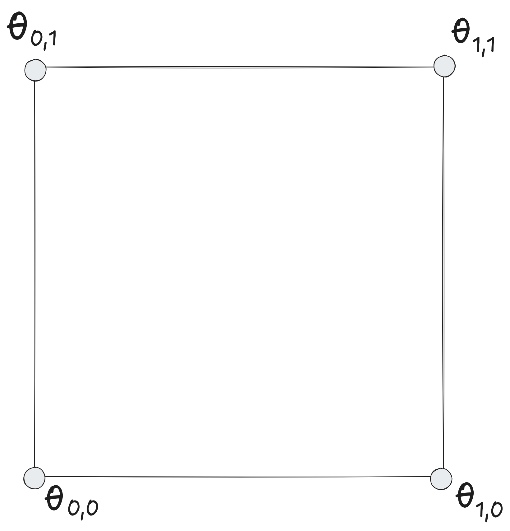
• Store \(Q(s,a)\) for a limited number of states: \(\theta(s,a)\)
• Weighting function \(\beta\)
  • Maps true states to states in \(\theta\)

\(Q(s,a) = \theta^T\beta(s,a)\)

Update step:

\(\theta \gets \theta + \alpha \left[R + \gamma \theta^T \beta(s', a') - \theta^T\beta(s, a)\right] \beta(s, a)\)

Linear Approximation Q-Learning

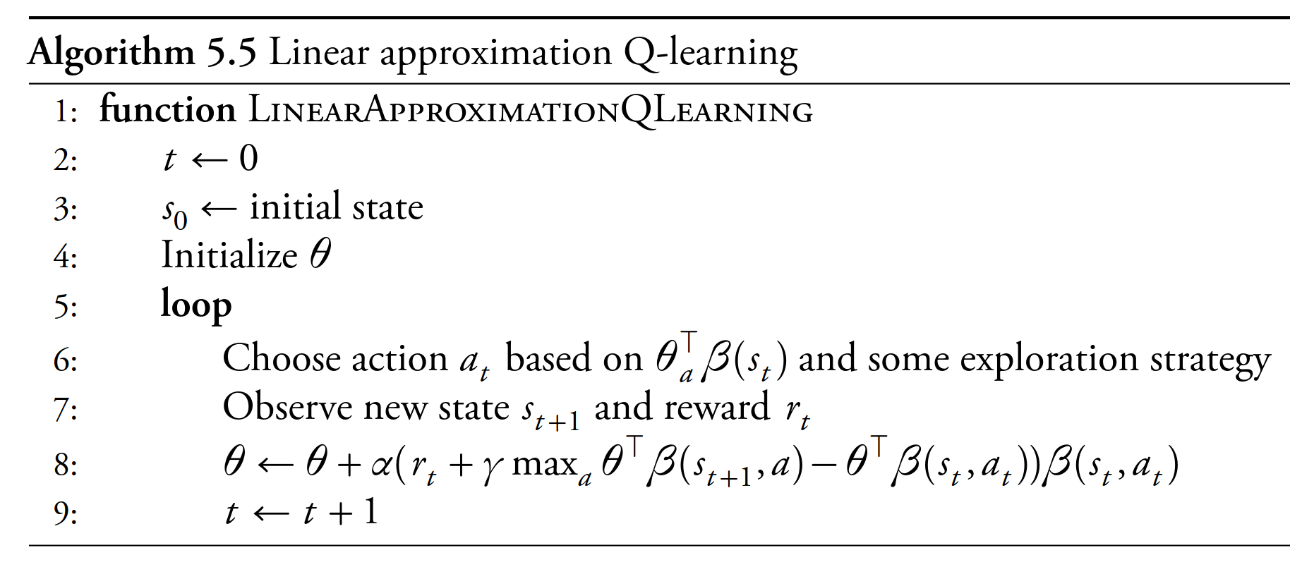Mykal Kochenderfer. Decision Making Under Uncertainty, MIT Press 2015

Example: Grid Interpolations

References

• Richard S. Sutton and Andrew G. Barto. Reinforcement Learning: An Introduction. 2nd Edition, 2018.

• Mykal Kochenderfer, Tim Wheeler, and Kyle Wray. Algorithms for Decision Making. 1st Edition, 2022.

• John G. Kemeny and J. Laurie Snell, Finite Markov Chains. 1st Edition, 1960.

• Stanford CS234 (Emma Brunskill)

• UCL Reinforcement Learning (David Silver)

• Stanford CS228 (Mykal Kochenderfer)