Review

CSCI 4511/6511

Joe Goldfrank

Announcements

• Final Exam: 25 Apr
• Project Milestone 1: 20 Apr
• Project Milestone 2: 27 Apr
• Homework Three:
  • Turn in for 75% credit max through 25 Apr (hard deadline)

Final Exam

• In class 25 Apr (next week!)
  • 120 minutes
  • 14 sides of notes (8.5”x11” or A4)
  • Final exam grade can replace midterm grade if higher
    • Midterm exam grade will not replace final exam grade
  • Calculators permitted
    • No networking capability

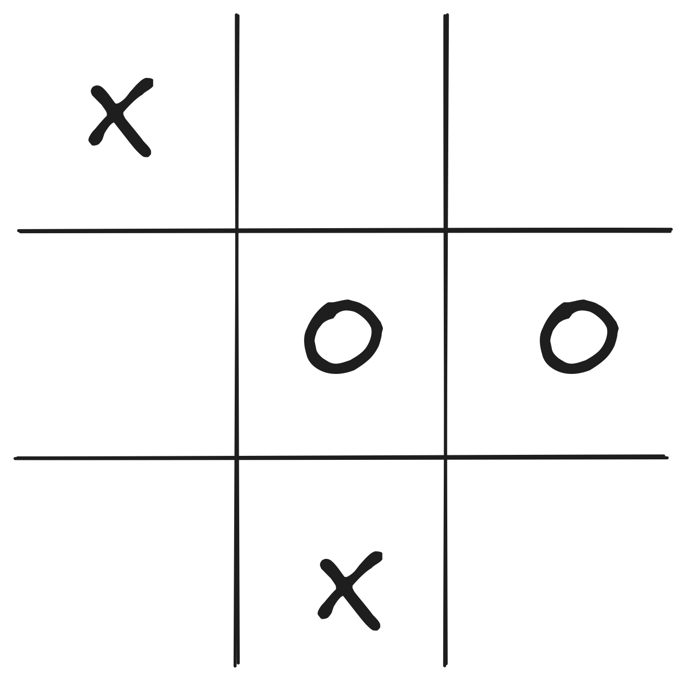
Reflex Agent

• Very basic form of agent function
• Percept \(\rightarrow\) Action lookup table
• Good for simple games
  • Tic-tac-toe
  • Checkers?
• Needs entire state space in table

Partially-Observable State

• Most real-world problems
  • Sensor error
  • Model error
• Reflex agents fail¹
• Agent needs a belief state

1. Unless total number of partial observations is bounded

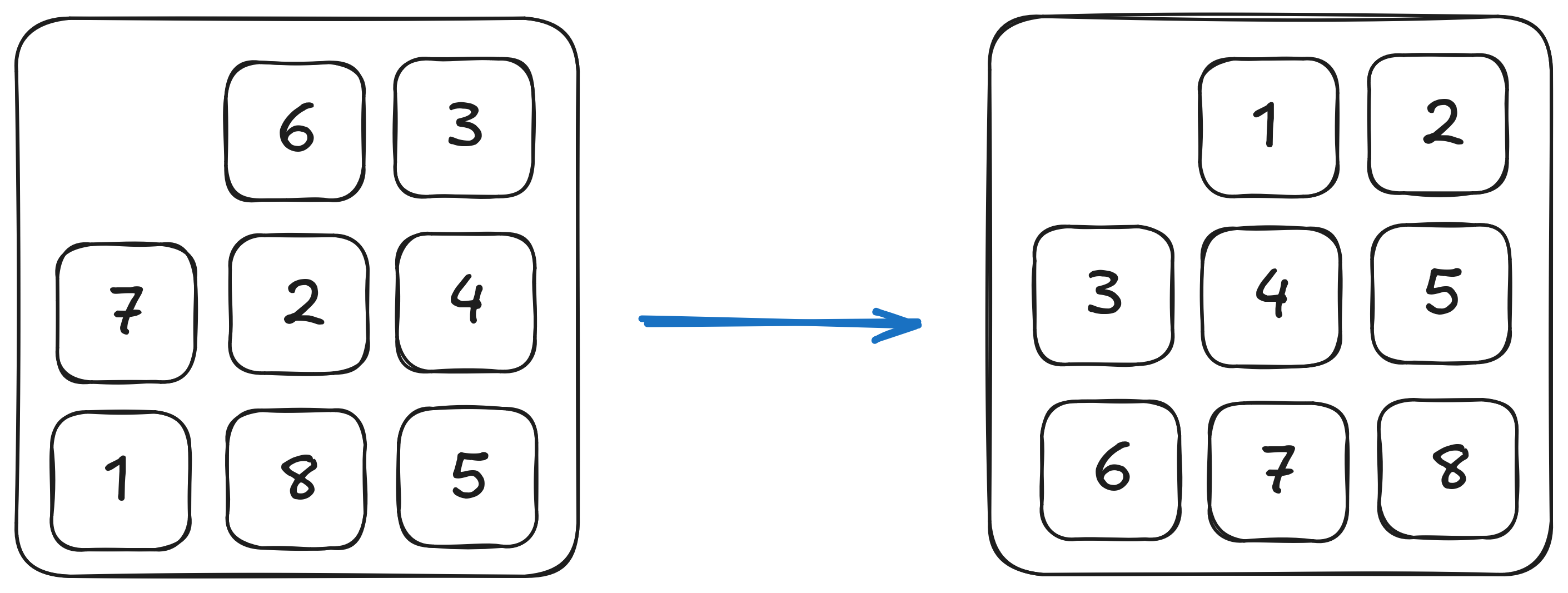
State

What is the state space?

Search: Why?

• Fully-observed problem
• Deterministic actions and state
• Well defined start and goal

Other Applications

• Route planning
• Protein design
• Robotic navigation
• Scheduling
  • Science
  • Manufacturing

Not Included

• Uncertainty
  • State transitions known
• Adversary
  • Nobody wants us to lose
• Cooperation
• Continuous state

Search Problem

Search problem includes:

• Start State
• State Space
• State Transitions
• Goal Test

State Space:

Actions & Successor States:

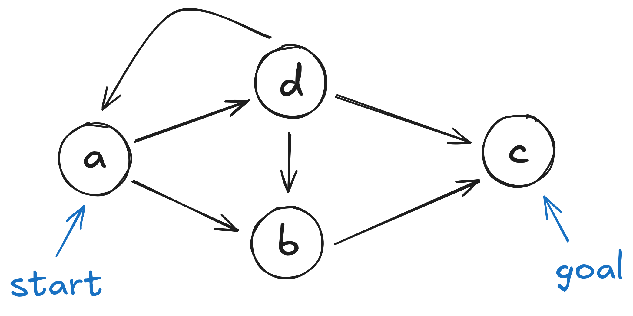
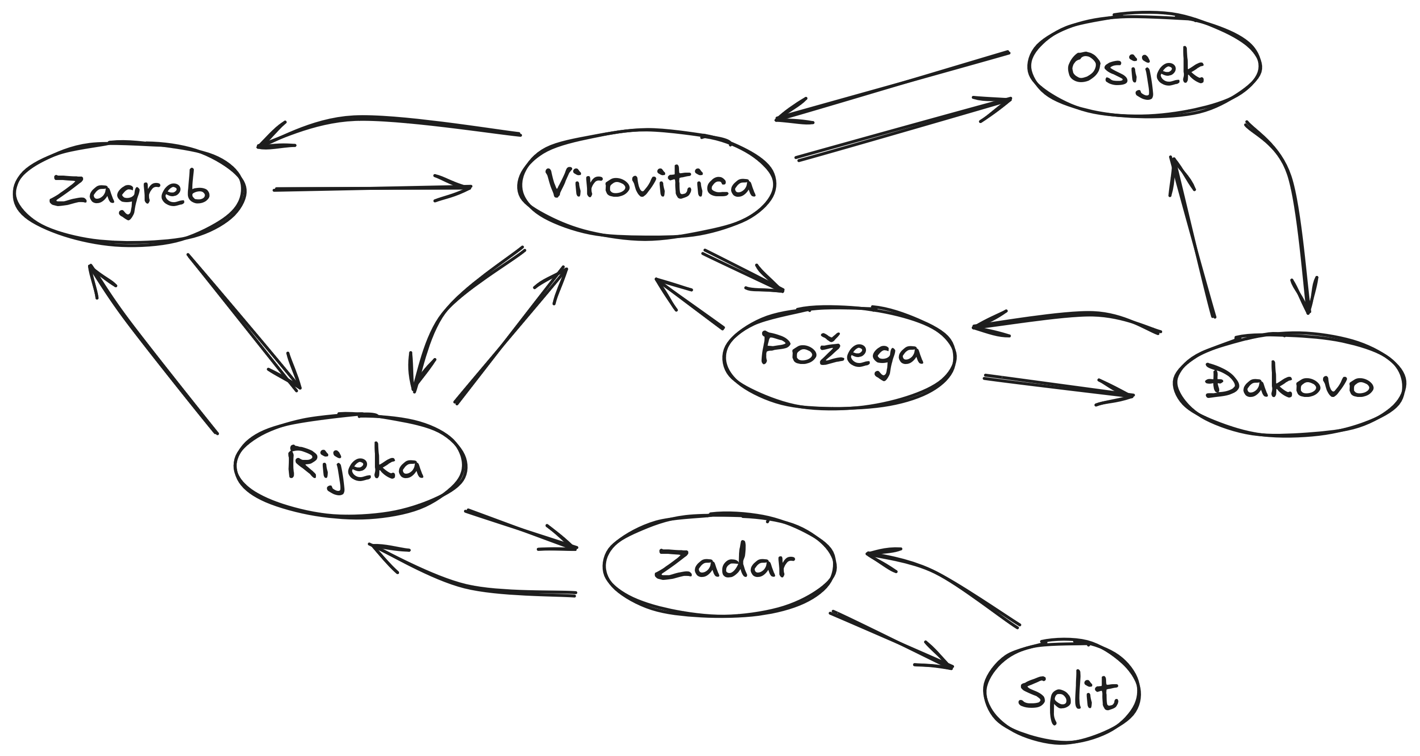
State Space Graph

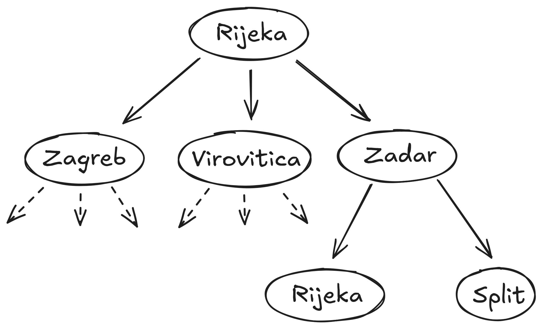
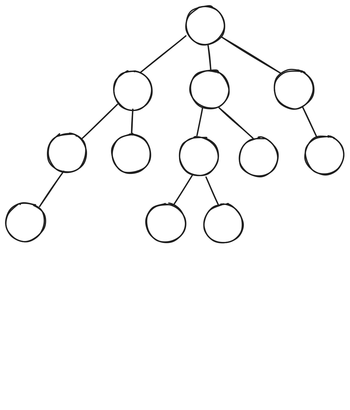
Search Trees

Graph:

Tree:

Let’s Talk About Trees

• For any non-trivial problem, they’re big
  • (Effective) branching factor
  • Depth
• Graph and tree both too large for memory
  • Successor function (graph)
  • Expansion function (tree)

How To Solve It

Given:

• Starting node
• Goal test
• Expansion

Do:

• Expand nodes from start
• Test each new node for goal
  • If goal, success
• Expand new nodes
  • If nothing left to expand, failure

Tree Search Algorithms

• BFS
• DFS
• UCS/Dijkstra
• A*
• Greedy searches

A* Search

• Include path-cost \(g(n)\)
  • \(f(n) = g(n) + h(n)\)
• Complete (always)
• Optimal (sometimes)
• Painful \(O(b^m)\) time and space complexity

Choosing Heuristics

• Recall: \(h(n)\) estimates cost from \(n\) to goal

• Admissibility
• Consistency

Choosing Heuristics

• Admissibility
  • Never overestimates cost from \(n\) to goal
  • Cost-optimal!
• Consistency
  • \(h(n) \leq c(n, a, n') + h(n')\)
  • \(n'\) successors of \(n\)
  • \(c(n, a, n')\) cost from \(n\) to \(n'\) given action \(a\)

Consistency

• Consistent heuristics are admissible
  • Inverse not necessarily true
• Always reach each state on optimal path

Weighted A* Search

• Greedy: \(f(n) = h(n)\)
• A*: \(f(n) = h(n) + g(n)\)
• Uniform-Cost Search: \(f(n) = g(n)\)

…

• Weighted A* Search: \(f(n) = W\cdot h(n) + g(n)\)
  • Weight \(W > 1\)

Iterative-Deepening A* Search

“IDA*” Search

• Similar to Iterative Deepening with Depth-First Search
  • DFS uses depth cutoff
  • IDA* uses \(h(n) + g(n)\) cutoff with DFS
  • Once cutoff breached, new cutoff:
    • Typically next-largest \(h(n) + g(n)\)
  • \(O(b^m)\) time complexity 😔
  • \(O(d)\) space complexity¹ 😌

1. This is slightly complicated based on heuristic branching factor \(b_h\).

Where Do Heuristics Come From?

• Intuition
  • “Just Be Really Smart”
• Relaxation
  • The problem is constrained
  • Remove the constraint
• Pre-computation
  • Sub problems
• Learning

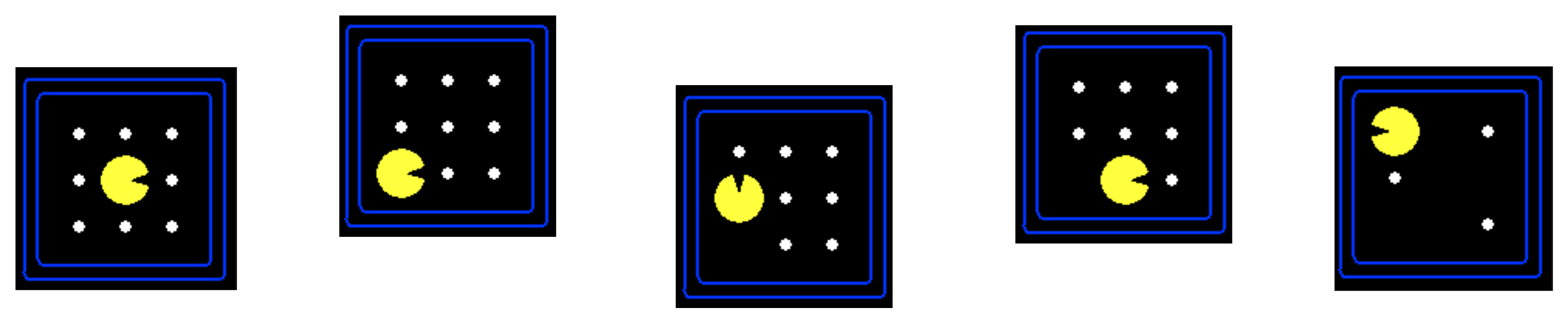
Local Search

Uninformed/Informed Search:

• Known start, known goal
• Search for optimal path

Local Search:

• “Start” is irrelevant
• Goal is not known
  • But we know it when we see it
• Search for goal

“Real-World” Examples

• Scheduling
• Layout optimization
  • Factories
  • Circuits
• Portfolio management
• Others?

Hill-Climbing

• Objective function
• State space mapping
  • Neighbors

Variations

• Sideways moves
  • Not free
• Stochastic moves
  • Full set
  • First choice
• Random restarts
  • If at first you don’t succeed, you fail try again!
  • Complete 😌

The Trouble with Local Maxima

• We don’t know that they’re local maxima
  • Unless we do?
• Hill climbing is efficient
  • But gets trapped
• Exhaustive search is complete
  • But it’s exhaustive!
  • Stochastic methods are ‘exhaustive’

Simulated Annealing

• Doesn’t actually have anything to do with metallurgy
• Search begins with high “temperature”
  • Temperature decreases during search
• Next state selected randomly
  • Improvements always accepted
  • Non-improvements rejected stochastically
  • Higher temperature, less rejection
  • “Worse” result, more rejection

Local Beam Search

Recall:

• Beam search keeps track of \(k\) “best” branches

Local Beam Search:

• Hill climbing search, keeping track of \(k\) successors
  • Deterministic
  • Stochastic

Simple Games

• Two-player
• Turn-taking
• Discrete-state
• Fully-observable
• Zero-sum
  • This does some work for us!

Minimax

• Initial state \(s_0\)
• Actions(\(s\)) and To-move(\(s\))
• Result(\(s, a\))
• Is-Terminal(\(s\))
• Utility(\(s, p\))

More Than Two Players

• Two players, two values: \(v_A, v_B\)
  • Zero-sum: \(v_A = -v_B\)
  • Only one value needs to be explicitly represented
• \(> 2\) players:
  • \(v_A, v_B, v_C ...\)
  • Value scalar becomes \(\vec{v}\)

Minimax Efficiency

Pruning removes the need to explore the full tree.

• Max and Min nodes alternate
• Once one value has been found, we can eliminate parts of search
  • Lower values, for Max
  • Higher values, for Min
• Remember highest value (\(\alpha\)) for Max
• Remember lowest value (\(\beta\)) for Min

Solving Non-Deterministic Games

Previously: Max and Min alternate turns

Now:

• Max
• Chance
• Min
• Chance

😣

Expectiminimax

Constraint Satisfaction

• Express problem in terms of state variables
  • Constrain state variables
• Begin with all variables unassigned
• Progressively assign values to variables
• Assignment of values to state variables that “works:” solution

More Formally

• State variables: \(X_1, X_2, ... , X_n\)
• State variable domains: \(D_1, D_2, ..., D_n\)
  • The domain specifies which values are permitted for the state variable
  • Domain: set of allowable variables (or permissible range for continuous variables)¹
  • Some constraints \(C_1, C_2, ..., C_m\) restrict allowable values

1. Or a hybrid, such as a union of ranges of continuous variables.

Constraint Types

• Unary: restrict single variable
  • Can be rolled into domain
  • Why even have them?
• Binary: restricts two variables
• Global: restrict “all” variables

Constraint Examples

• \(X_1\) and \(X_2\) both have real domains, i.e. \(X_1, X_2 \in \mathbb{R}\)
  • A constraint could be \(X_1 < X_2\)
• \(X_1\) could have domain \(\{\text{red}, \text{green}, \text{blue}\}\) and \(X_2\) could have domain \(\{\text{green}, \text{blue}, \text{orange}\}\)
  • A constraint could be \(X_1 \neq X_2\)
• \(X_1, X_2, ..., X_100 \in \mathbb{R}\)
  • Constraint: exactly four of \(X_i\) equal 12
  • Rewrite as binary constraint?

Assignments

• Assignments must be to values in each variable’s domain
• Assignment violates constraints?
  • Consistency
• All variables assigned?
  • Complete

Graph Representation I

Constraint graph: edges are constraints

Graph Representation II

Constraint hypergraph: constraints are nodes

Solving CSPs

• We can search!
  • …the space of consistent assignments
• Complexity \(O(d^n)\)
  • Domain size \(d\), number of nodes \(n\)
• Tree search for node assignment
  • Inference to reduce domain size
• Recursive search

Inference

• Arc consistency
  • Reduce domains for pairs of variables
• Path consistency
  • Assignment to two variables
  • Reduce domain of third variable

Ordering

• Select-Unassgined-Variable(\(CSP, assignment\))
  • Choose most-constrained variable¹
• Order-Domain-Variables(\(CSP, var, assignment\))
  • Least-constraining value

• Tree-structure: Linear time solution

1. or MRV: “Minimum Remaining Values”

Logic

• \(\neg\)
  • “Not” operator, same as CS (!, not, etc.)
• \(\land\)
  • “And” operator, same as CS (&&, and, etc.)
  • This is sometimes called a conjunction.
• \(\lor\)
  • “Inclusive Or” operator, same as CS.
  • This is sometimes called a disjunction.

Unfamiliar Logical Operators

• \(\Rightarrow\)
  • Logical implication.
    
  • If \(X_0 \Rightarrow X_1\), \(X_1\) is always True when \(X_0\) is True.
    
  • If \(X_0\) is False, the value of \(X_1\) is not constrained.
• \(\iff\)
  • “If and only If.”
  • If \(X_0 \iff X_1\), \(X_0\) and \(X_1\) are either both True or both False.
  • Also called a biconditional.

Knowledge Base & Queries

• We encode everything that we ‘know’
  • Statements that are true
• We query the knowledge base
  • Statement that we’d like to know about
• Logic:
  • Is statement consistent with KB?

Entailment

• \(KB \models A\)
  • “Knowledge Base entails A”
  • For every model in which \(KB\) is True, \(A\) is also True
  • One-way relationship: \(A\) can be True for models where \(KB\) is not True.
• Vocabulary: \(A\) is the query

Knowing Things

Falsehood:

• \(KB \models \neg A\)
  • No model exists where \(KB\) is True and \(A\) is True

It is possible to not know things:¹

• \(KB \nvdash A\)
• \(KB \nvdash \neg A\)

1. \(\nvdash\) – “does not entail”

Conjunctive Normal Form

• Literals — symbols or negated symbols
  • \(X_0\) is a literal
  • \(\neg X_0\) is a literal
• Clauses — combine literals and disjunction using disjunctions (\(\lor\))
  • \(X_0 \lor \neg X_1\) is a valid disjunction
  • \((X_0 \lor \neg X_1) \lor X_2\) is a valid disjunction

Conjunctive Normal Form

• Conjunctions (\(\land\)) combine clauses (and literals)
  • \(X_1 \land (X_0 \lor \neg X_2)\)
• Disjunctions cannot contain conjunctions:
• \(X_0 \lor (X_1 \land X_2)\) not in CNF
  • Can be rewritten in CNF: \((X_0 \lor X_1) \land (X_0 \lor X_2)\)

Converting to CNF

• \(X_0 \iff X_1\)
  • \((X_0 \Rightarrow X_1) \land (X_1 \Rightarrow X_0)\)
• \(X_0 \Rightarrow X_1\)
  • \(\neg X_0 \lor X_1\)
• \(\neg (X_0 \land X_1)\)
  • \(\neg X_0 \lor \neg X_1\)
• \(\neg (X_0 \lor X_1)\)
  • \(\neg X_0 \land \neg X_1\)

Joint Distributions

• Distribution over multiple variables
  • \(P(x, y)\) represents \(P\{X=x, Y=y\}\)
• Marginal distribution:
  • \(P(x) = \sum_y P(x,y)\)

Independence

Conditional probability:

\[P(x | y) = \frac{P(x, y)}{P(y)}\]

Bayes’ rule:

\[P(x | y) = \frac{P(y | x)P(x)}{P(y)} \]

Conditional Independence

\[P(x | y) = P(x) \rightarrow P(x,y) = P(x) P(y)\]

• Two variables can be conditionally independent…
  • … when conditioned on a third variable

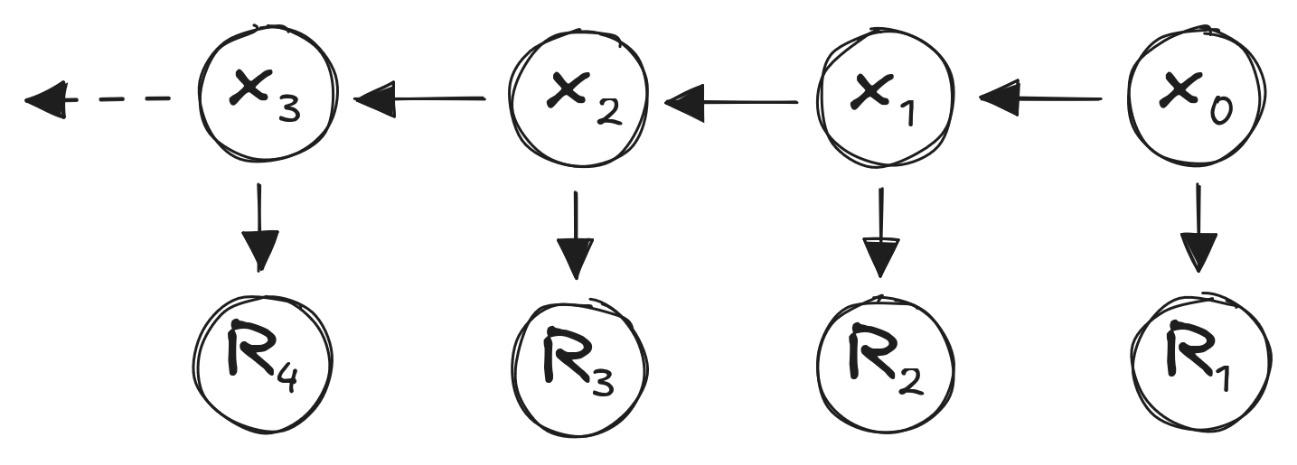
Markov Chains

Markov property:

\(P(X_{t} | X_{t-1},X_{t-2},...,X_{0}) = P(X_{t} | X_{t-1})\)

“The future only depends on the past through the present.”

• State \(X_{t-1}\) captures “all” information about past
• No information in \(X_{t-2}\) (or other past states) influences \(X_{t}\)

State Transitions

Stochastic matrix \(P\)

\[ P = \begin{bmatrix} P_{1,1} & \dots & P_{1,n}\\ \vdots & \ddots & \\ P_{n, 1} & & P_{n,n} \end{bmatrix} \]

• All rows sum to 1
• Discrete state spaces implied

Stationary Behavior

• “Long run” behavior of Markov chain

\(x_0 P^k\) for large \(k\)

• “Stationary state” \(\pi\) such that:

\(\pi = \pi P\)

• Row eigenvector for \(P\) for eigenvalue 1
• 😌

Absorbing States

• State that cannot be “escaped” from
  • Example: gambling \(\rightarrow\) running out of money

\(P = \begin{bmatrix} 0.5 & 0.3 & 0.1 & 0.1 \\ 0.3 & 0.4 & 0.3 & 0 \\ 0.1 & 0.6 & 0.2 & 0.1 \\ 0 & 0 & 0 & 1 \end{bmatrix}\)

• Non-absorbing states: “transient” states

Markov Reward Process

• Reward function \(R_s = E[R_{t+1} | S_t = s]\):
  • Reward for being in state \(s\)
• Discount factor \(\gamma \in [0, 1]\)

\(U_t = \sum_k \gamma^k R_{t+k+1}\)

The Markov Decision Process

• Transition probabilities depend on actions

Markov Process:

\(s_{t+1} = s_t P\)

Markov Decision Process (MDP):

\(s_{t+1} = s_t P^a\)

Rewards: \(R^a\) with discount factor \(\gamma\)

MDP - Policies

• Agent function
  • Actions conditioned on states

\(\pi(s) = P[A_t = a | s_t = s]\)

• Can be stochastic
  • Usually deterministic
  • Usually stationary

MDP - Policies

State value function \(U^\pi\):¹

\(U^\pi(s) = E_\pi[U_t | S_t = s]\)

State-action value function \(Q^\pi\):²

\(Q^\pi(s,a) = E_\pi[U_t | S_t = s, A_t = a]\)

Notation: \(E_\pi\) indicates expected value under policy \(\pi\)

1. Often simply called “value function”

2. Often simply called “action value function”

Bellman Expectation

Value function:

\(U^\pi(s) = E_\pi[R_{t+1} + \gamma U^\pi (S_{t+1}) | S_t = s]\)

Action-value fuction:

\(Q^\pi(s, a) = E_\pi[R_{t+1} + \gamma Q^\pi(S_{t+1}, A_{t+1}) | S_t = s, A_t =a]\)

Bellman Equation

\[U^*(s) = \max_a R(s, a) + \gamma \sum \limits_{s'} T(s' | s, a) U^*(s')\]

Bellman Equation

\[Q^*(s, a) = R(s, a) + \gamma \sum \limits_{s'} T(s' | s, a) \max_a Q^*(s', a')\]

How To Solve It

• No closed-form solution
  • Optimal case differs from policy evaluation

Iterative Solutions:

• Value Iteration
• Policy Iteration

Reinforcement Learning:

• Q-Learning
• Sarsa

Model Uncertainty

Action-value function:

\(Q(s, a) = R(s, a) + \gamma \sum \limits_{s'} T(s' | s, a) U(s')\)

we don’t know \(T\):

\(U^\pi(s) = E_\pi \left[ r_t + \gamma r_{t+1} + \gamma^2 r_{t+2} + \gamma^3 r_{t+3} + ...|s \right]\)

\(Q(s, a) = E_\pi \left[ r_t + \gamma r_{t+1} + \gamma^2 r_{t+2} + \gamma^3 r_{t+3} + ...|s,a \right]\)

Temporal Difference (TD) Learning

• Take action from state, observe new state, reward

\(U(s) \gets U(s) + \alpha \left[ r + \gamma U(s') - U(s)\right]\)

• Update immediately given \((s, a, r, s')\)

• TD Error: \(\left[ r + \gamma U(s') - U(s)\right]\)
  • Measurement: \(r + \gamma U(s')\)
  • Old Estimate: \(U(s)\)

RL Methods

• Q-Learning
• Sarsa
• Eligibility traces

RL Methods

Q-Learning:
\(\quad \quad Q(s,a) \gets Q(s,a) +\alpha \left[R + \gamma \max \limits_{a'} Q(s', a') - Q(s,a)\right]\)

Sarsa:
\(\quad \quad Q(s,a) \gets Q(s,a) +\alpha \left[R + \gamma Q(s', a') - Q(s,a)\right]\)

Sarsa-\(\lambda\):
\(\quad \quad \delta = R + \gamma Q(s',a') - Q(s,a)\) \(\quad \quad Q(s,a) \gets \alpha \delta N(s,a)\)

Monte Carlo Tree Search - Search

• If current state \(\in T\) (tree states):

  • Maximize: \(Q(s,a) + c\sqrt{\frac{\log N(s)}{N(s,a)}}\)
  • Update \(Q(s,a)\) during search

Monte Carlo Tree Search - Expansion

• State \(\notin T\)
  • Initialize \(N(s,a)\) and \(Q(s,a)\)
  • Add state to \(T\)

Monte Carlo Tree Search - Rollout

• Policy \(\pi_0\) is “rollout” policy
  • Usually stochastic
  • States not tracked

References

• Stuart J. Russell and Peter Norvig. Artificial Intelligence: A Modern Approach. 4th Edition, 2020.

• Richard S. Sutton and Andrew G. Barto. Reinforcement Learning: An Introduction. 2nd Edition, 2018.

• Mykal Kochenderfer, Tim Wheeler, and Kyle Wray. Algorithms for Decision Making. 1st Edition, 2022.

• UC Berkeley CS188

• Stanford CS234 (Emma Brunskill)

• Stanford CS228 (Mykal Kochenderfer)