Markov Decision Processes

This example shows a very simple application of the dynamic programing using three related algorithms: Synchronous Value Iteration, Policy Iteration, and Asynchronous Value Iteration.

We’ll solve a problem (determine an optimal policy) similar to the example in last week’s lecture.

Imports:

import numpy as np
import polars as pl
import seaborn as sns
from copy import deepcopy
sns.set_theme(style="whitegrid")

Problem Setup

Similar to last week’s lecture, but slightly more complicated: the problem consists of four states and three actions.

Each state represents a sales volume (low, med-low, med-high, and high), and each action represents how much is spent on advertising.

Note how when more is spent on advertising, the next state is generally more likely to be a higher sales volume.

\(P^0 = \begin{bmatrix}0.5 & 0.4 & 0.1 & 0 \\ 0.4 & 0.5 & 0.1 & 0 \\ 0.7 & 0.1 & 0.1 & 0.1 \\ 0.5 & 0.2 & 0.2 & 0.1 \end{bmatrix} \quad P^1 = \begin{bmatrix} 0.7 & 0.2 & 0.0 & 0.1 \\ 0.2 & 0.3 & 0.4 & 0.1 \\ 0.5 & 0.2 & 0.2 & 0.1 \\ 0.4 & 0.2 & 0.2 & 0.1 \end{bmatrix} \quad P^2 = \begin{bmatrix} 0.1 & 0.3 & 0.4 & 0.2 \\ 0.1 & 0.3 & 0.5 & 0.1 \\ 0.3 & 0.3 & 0.1 & 0.3 \\ 0.3 & 0.4 & 0.1 & 0.2 \end{bmatrix}\)

\(R^0 = \begin{bmatrix} 1 \\ 3 \\ 5 \\ 12 \end{bmatrix} \quad R^1 = \begin{bmatrix} 0 \\ 2 \\ 4 \\ 11 \end{bmatrix} \quad R^2 = \begin{bmatrix} -2 \\ 0 \\ 2 \\ 9 \end{bmatrix} \quad \gamma = 0.95\)

P0 = np.array([[0.5, 0.4, 0.1, 0],
               [0.4, 0.5, 0.1, 0],
               [0.7, 0.1, 0.1, 0.1],
               [0.5, 0.2, 0.2, 0.1]
              ])

P1 = np.array([[0.7, 0.2, 0.0, 0.1],
               [0.2, 0.3, 0.4, 0.1],
               [0.5, 0.2, 0.2, 0.1],
               [0.4, 0.2, 0.2, 0.2]
              ])

P2 = np.array([[0.1, 0.3, 0.4, 0.2],
               [0.1, 0.3, 0.5, 0.1],
               [0.3, 0.3, 0.1, 0.3],
               [0.3, 0.4, 0.1, 0.2]
              ])

R0 = np.array([[1],[3], [5], [12]])

R1 = np.array([[0],[2], [4], [11]])

R2 = np.array([[-2],[0], [2], [9]])

states = [np.array([[1, 0, 0, 0]]), 
          np.array([[0, 1, 0, 0]]), 
          np.array([[0, 0, 1, 0]]), 
          np.array([[0, 0, 0, 1]])]

# transition and reward as 'function'  of action
# represented as dicts
T = {0: P0, 1: P1, 2: P2}
R = {0: R0, 1: R1, 2: R2}

gamma = 0.95

Policy Evaluation

Bellman backup for iterative policy evaluation:

\(U^\pi_{k+1}(s) = R(s, \pi(s)) + \gamma \sum \limits_{s^{'}} T(s' | s, \pi(s)) U_k^\pi(s')\)

Implemented below using functions for each transition. We could also use matrix multiplication, but the functions are easier to read and understand.

# returns Q for one state
def bellman_backup(s, U, pi, gamma, T=T, R=R, S=states):
    action = pi[s]
    reward = R[action][s]
    sum = 0
    for s_prime in range(len(S)):
        sum += T[action][s][s_prime] * U[s_prime]
    sum *= gamma
    return (reward + sum)[0]

Policy Update

Given:

\(Q^*(s, a) = R(s, a) + \gamma \sum \limits_{s'} T(s' | s, a) U^*(s')\)

Again, implemented as a “function” rather than using matrix multiplication.

def Q_sa(s, a, U, pi, gamma, T=T, R=R):
    action = a
    reward = R[action][s]
    sum = 0
    for s_prime in range(len(states)):
        sum += T[a][s][s_prime] * U[s_prime]
    sum *= gamma
    return (reward + sum)[0]

Synchronous Value Iteration

Initializing values and policy

pi = {0:0, 1:0, 2:0, 3:0} # initial policy
U = np.array([0.0 for _ in range(len(states))]) # initial values

# for implementation
U_vals = [[u] for u in U] # store U values
old_U = U - 0.1 # to start loop

Value iteration algorithm

We select policy according to \(U_{k+1}(s) = \max_a Q(s,a)\), then update \(U^\pi\) and iterate until convergence.

We run the algorithm until utility converges within some \(\epsilon\), chosen here as \(0.01\).

# iterate until values converge within 0.01
iterations = 0
while np.sum(U-old_U) > 0.01:
    iterations += 1
    Q = {}
    new_pi = {}
    # update policy based on U values
    for s in range(len(states)): # iterate over all states
        argmax_a = None
        max_Q = -1*float('inf')
        
        for a in range(len(T)): # iterate over possible actions
            Q[(s,a)] = Q_sa(s, a, U, pi, gamma) # calculate Q-value
            if Q[(s,a)] > max_Q: # get max, argmax
                argmax_a = a
                max_Q = Q[(s,a)]
        new_pi[s] = argmax_a # update policy for state
    pi = new_pi # update full policy
    
    # update values
    old_U = deepcopy(U) # keep old value to determine convergence
    U = [bellman_backup(i, U, pi, gamma) for i in range(len(states))]
    U = np.array(U)
    
    # for plotting
    for i, u in enumerate(U):
        U_vals[i].append(u)

U_value_iteration = U
print("Policy:", pi)
print("Total Iterations:", iterations)

Policy: {0: 2, 1: 1, 2: 0, 3: 1}
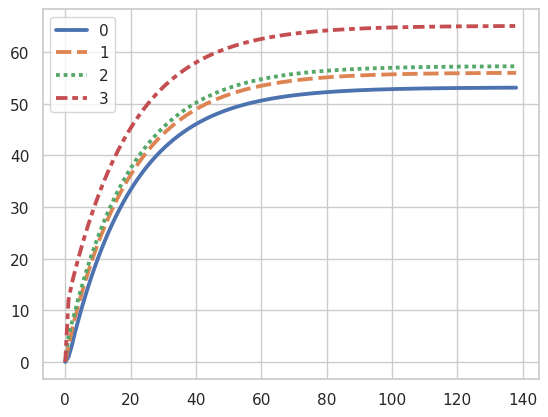
Total Iterations: 138

Plotting Value Convergence

df = pl.DataFrame(U_vals, schema=[f"U_{i}" for i, u in enumerate(U)])
sns.lineplot(df, linewidth=2.75, legend='full')

Policy Iteration

Initializing values and policy

pi = {0:0, 1:0, 2:0, 3:0} # initial policy
old_pi = None
U = np.array([0.0 for _ in range(len(states))]) # initial values

# for implementation
U_vals = [[u] for u in U] # store U values
old_U = U - 0.1 # to start loop

print(pi)
iterations = 0
while pi != old_pi:
    # determine U of policy
    # iterate until values converge within 0.01
    while np.sum(U-old_U) > 0.01:
        iterations += 1
        old_U = deepcopy(U)
        U = np.array([bellman_backup(i, U, pi, gamma) for i in range(len(states))])
        # for plotting
        for i, u in enumerate(U):
            U_vals[i].append(u)
    
    # extract policy from U values
    Q = {}
    new_pi = {}
    for s in range(len(states)): # iterate over all states
        argmax_a = None
        max_Q = -1*float('inf')

        for a in range(len(T)): # iterate over possible actions
            Q[(s,a)] = Q_sa(s, a, U, pi, gamma) # calculate Q-value
            if Q[(s,a)] > max_Q: # get max, argmax
                argmax_a = a
                max_Q = Q[(s,a)]
        new_pi[s] = argmax_a # update policy for state
    old_pi = deepcopy(pi)
    pi = new_pi # update full policy
    U = [bellman_backup(i, U, pi, gamma) for i in range(len(states))]
    U = np.array(U)
    print("Policy:", pi)
    print("Total Iterations:", iterations)

U_policy_iteration = U

{0: 0, 1: 0, 2: 0, 3: 0}
Policy: {0: 2, 1: 1, 2: 0, 3: 1}
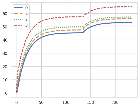
Total Iterations: 135
Policy: {0: 2, 1: 1, 2: 0, 3: 1}
Total Iterations: 234

Plotting Value Convergence

df = pl.DataFrame(U_vals, schema=[f"U_{i}" for i, u in enumerate(U)])
sns.lineplot(df, linewidth=2.75, legend='full')

Asynchronous Value Iteration

pi = {0:0, 1:0, 2:0, 3:0} # initial policy
U = np.array([0.0 for _ in range(len(states))]) # initial values

# for implementation
U_vals = [[u] for u in U] # store U values
old_U = U - 0.1 # to start loop

# iterate until values converge within 0.01
iterations = 0
while np.sum(U-old_U) > 0.01:
    iterations += 1
    Q = {}
        
    s = np.argmax(U-old_U) # choose s according to some rule
    
    argmax_a = None
    max_Q = -1*float('inf')
    for a in range(len(T)): # iterate over possible actions
        Q[(s,a)] = Q_sa(s, a, U, pi, gamma) # calculate Q-value
        if Q[(s,a)] > max_Q: # get max, argmax
            argmax_a = a
            max_Q = Q[(s,a)]
    pi[s] = argmax_a # update policy for state

    # update values
    old_U = deepcopy(U) 
    U = np.array([bellman_backup(i, U, pi, gamma) for i in range(len(states))])
    
    # for plotting
    for i, u in enumerate(U):
        U_vals[i].append(u)

U_async_val_iteration = U
print("Policy:", pi)
print("Total Iterations:", iterations)

Policy: {0: 2, 1: 1, 2: 0, 3: 1}
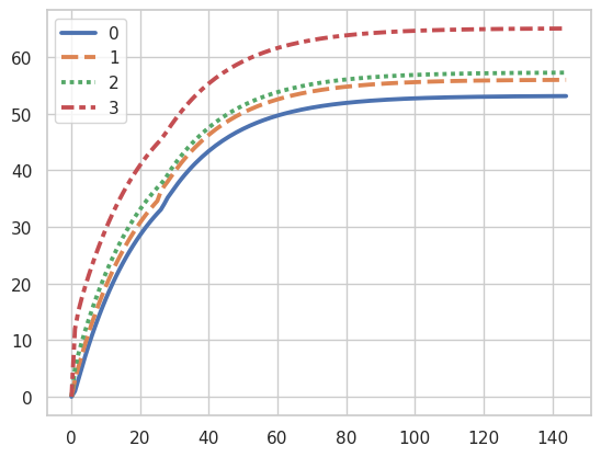
Total Iterations: 144

Plotting Value Convergence

df = pl.DataFrame(U_vals, schema=[f"U_{i}" for i, u in enumerate(U)])
sns.lineplot(df, linewidth=2.75, legend='full')

These algorithms all ultimately solve for an optimal policy using the Bellman equation, so we find that the utilities and policies from each will be the same.

print(U_value_iteration)
print(U_policy_iteration)
print(U_async_val_iteration)

[53.13439528 56.00000181 57.27536126 65.07537912]
[53.13694775 56.00255428 57.27791374 65.07793159]
[53.13407081 55.99967735 57.2750368  65.07505466]